Research Article | | Peer-Reviewed

Geospatial Modeling of Urban Sprawl in Bharatpur Metropolitan City

Received: 3 September 2025     Accepted: 13 January 2026     Published: 28 April 2026
Views:       Downloads:
Abstract

Rapid socioeconomic developments have spurred urban sprawl in Nepal. Bharatpur Metropolitan City (BMC) in recent decades, resulting in notable changes to the land use and environment. Using Landsat images and GIS-based methods, this study examines the spatial and temporal dynamics of urban sprawl from 1990 to 2020 and projects future growth through 2040. Built-up areas expanded by over 20 times, from 3.29 km2 in 1990 to 64.32 km2 in 2020, according to the Land Use and Land Cover (LULC) categorization. At the same time, there was a significant amount of land conversion as agricultural land decreased from 221.88 km2 to 193.90 km2 and barren land decreased by more than 60%. Three predominant types of urban sprawl were found: leapfrog (important within 0–30 km buffers), infill (8.94 km2), and extension (103.48 km2). The most common areas for extension-type sprawl were those between 0 and 5 km. Built-up area is expected to rise by 132% from 2020 levels to 113.25 km2 by 2030 and 149.33 km2 by 2040, according to spatiotemporal analysis and CA-Markov modelling. By 2040, this growth is expected to further reduce the amount of agricultural land to 118.78 km2. These results underline how urgently urban planning interventions are needed to manage haphazard development, protect arable land, and direct sustainable growth. The study shows how important it is to combine predictive modelling, spatial analysis, and remote sensing to inform land use regulations in areas that are rapidly becoming more urbanized.

Published in Urban and Regional Planning (Volume 11, Issue 2)
DOI 10.11648/j.urp.20261102.11
Page(s) 96-109
Creative Commons

This is an Open Access article, distributed under the terms of the Creative Commons Attribution 4.0 International License (http://creativecommons.org/licenses/by/4.0/), which permits unrestricted use, distribution and reproduction in any medium or format, provided the original work is properly cited.

Copyright

Copyright © The Author(s), 2026. Published by Science Publishing Group

Keywords

Urban Sprawl, LULC, RS and GIS, CA-Markov Modeling, Bharatpur Metropolitan City

1. Introduction
Urban sprawl is an unplanned and uneven growth pattern, resulting from various processes and inefficient resource utilization . Urban sprawl expansion is a significant issue in urban areas due to inadequate infrastructure and basic facilities like water supply, electricity, and sanitation services . Nepal has experienced rapid urbanization and population growth in the last six decades, largely due to the development of physical infrastructure and increased migration and population . Nepal's urbanization has significantly increased in recent years, making it one of the world's least urbanized countries and one of the top ten fastest-urbanizing nations . Nepal is grappling with climate change issues such as precipitation patterns, glacial melt timing, and rates, which could potentially affect agriculture, biodiversity, and hydropower energy production . Bharatpur, Nepal's administrative center, is a major commercial and service center known for its high-quality education, healthcare, and transportation. Located in the Terai region, it is situated in the Gandaki River drainage basin and has a modest watershed border with India . This research uses RS and GIS techniques to study the urban sprawl in Bharatpur metropolitan city from 1990 – 2020, focusing on the Kathmandu Valley, Pokhara Valley, Inner Terai valleys, and market and border towns located on highway junctures. Urban growth centers are emerging near the Indian border . Antalyn & Weerasinghe's study uses Landsat-8 OLI/TIRS and Landsat-5 TM satellite images to determine urban sprawl, Land Use Land Cover change, highlighting its unplanned, uneven growth patterns and inefficient resource utilization. Urban sprawl assessment has been utilized in various applied sciences, as demonstrated by Rimal et al. research on the Nepal Earthquake 2015's impact on urban growth in Kathmandu Valley. Shao et al. conducted a study on the impact of urban sprawl on sustainable development using remote sensing and social media data. Almeida utilized GIS and neighborhood statistics to analyze urban sprawl in Richmond, Virginia, identifying three density development types and setting threshold values. Gervasoni et al utilized three primary dimensions of sprawl: dispersion, land use mix, and accessibility, each requiring a specific numerical index computation. Falah et al. practiced Cellular automata (CA) as computational method for urban growth modelling. Litman suggests a comprehensive urban sprawl assessment that takes into account factors like development density, mix, centricity, transport network connectivity, and the quality of transport options. Suwal emphasizes the need for a robust and accountable governance structure to effectively manage and regulate urban growth in major cities, local areas, and newly expanded areas. Rapid urban growth's impact on environmental issues is a crucial concern for urban planners, policymakers, and environmentalists in these regions . This study examines social, demographic, and economic aspects of urban growth in BMC, including water supply, sanitation, health, housing patterns, and environmental infrastructure. It uses socio-economic data, urban base maps, GIS, and ERDAS imagery to analyze land use, land cover, socio-economic disparities, and environmental issues. The main objectives include analyzing spatial and temporal dynamics of land use, land suitability, impacts of urban growth on agricultural land, and the interaction between municipal water supply, sewage disposal, and environment.
1.1. Causes of Urban Sprawl
Urban sprawl is primarily driven by socioeconomic and cultural factors, with land value playing a significant role in rapid urban growth, often occurring in areas with lower property values . Three underlying forces that are interrelated with land values to increase the spatial urban sprawl . These forces are (i) Population growth in the periphery of central urban areas (ii) Rising income of people (iii) Third, decreasing commuting costs due to historical investment in transport infrastructure . This study explores the impact of labor migration in Nepal's hills, focusing on the effects on land management and the impact on households due to the resulting labor shortage, highlighting the ongoing emigration trend . Land use changes are influenced by human and environmental factors, and understanding their interplay can provide insights into actual changes and concessions . Land prices in rural and sub-urban areas are lower, and many Nepalese people work abroad, earning more money. This has led to increased land fragmentation in urban areas. Many people purchase small plots of land for residential purposes on the outskirts of metropolitan cities. As development increases infrastructure, residents' demands for transport, health, and education facilities increase. Land developers and real estate developers use these facilities to develop residential areas outside the city center . Technology and service centers are significant indicators of urbanization and urban sprawl. Computers reduce human relationships and improve quality at low costs. Developers and contractors use computer technology in urban development. Age plays a crucial role in urban sprawl patterns, with younger families seeking affordable housing options at the urban fringe. . That why urban sprawl cannot be defined by a single parameter . Galster et al. define urban sprawl as a pattern of land use and land cover, exhibiting eight dimensions: density, continuity, concentration, clustering, centrality, nuclearity, mixed uses, and proximity. The eight attributes of compacity/sprawl characterization combine physical and functional dimensions, focusing on the spatial configuration of land use development, density, and daily activity mix. Despite its unsustainable nature, people prefer larger lots in suburban communities, highlighting the importance of considering these dimensions when available information .
1.2. Consequences of Urban Sprawl
Urban sprawl's long-term impact, despite the significant single-family home construction, is difficult to predict over a longer period argue that the misconception of sprawl as offering affordable housing and a better quality of life is often misunderstood, leading to overlooked cumulative urban development impacts. refer to urban sprawl as the 'pitfall of marginalization', characterized by negative impacts such as crowding, accessibility, agricultural land degradation, and poor social infrastructure. Urban sprawl impacts infrastructure, utilities, and services efficiency, directly affecting people's livelihoods, property values, and commuting, and affecting various aspects of the urban environment . Urbanization, characterized by the expansion of impervious surfaces and the blocking of river or stream channels, is expected to increase flood vulnerability and risk. highlights the environmental impacts of urban sprawl, including air and water pollution, loss of natural habitats, reduced open space, increased flood risks, and reduced quality of life due to automobile dependence. In the 2000s, road network plans led to the expansion of building areas on major roads connecting the outskirts to five municipalities, replacing productive farmland . The reliance on automobiles, in particular, has contributed to the deterioration of air and water quality as well as the rapid depletion of fossil resources . New urban models offer insights into South Asian urban dynamics, but understanding physical and socioeconomic patterns remains limited. Geospatial technology fills this gap, but empirical case studies remain scarce .
1.3. Types of Urban Sprawl
Urban sprawl can vary across countries and contexts, with three distinct types of urban growth: newly grown, pre-growth, and newly developed . The study identifies three growth types: infilling, edge expansion, and spontaneous growth, each with varying importance in explaining the evolution of landscape patterns over time . The Landscape Expansion Index value determines if a growth patch is infilling, edge expansion, or spontaneous growth, indicating the three types of urban growth. According to Xu et al. each type of growth has a different level of dominance in the population. The hypothetical sequence of the spatial evolution of an urban area is shown below in Figure 1.
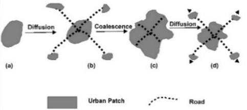
Figure 1. Hypothetical sequence of the spatial evolution of an urban area.
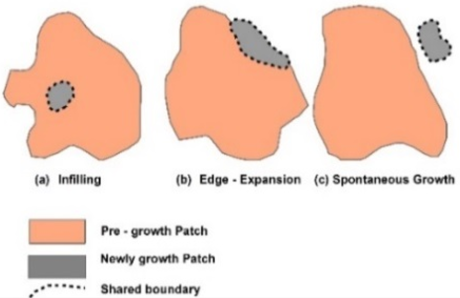
Figure 2. Three urban growth types.
Characterization of agricultural to urban landscape transition patterns and processes in Hanoi used a hypothetical model of spatial evolution . The urban land area grows as a result of diffusion and coalescence in the spatial evolution model (Figure 1). When new developments are built on the outskirts of an urban core, the once-compact landscape (Figure 1a) becomes increasingly fragmented (Figure 1b). They start to aggregate as they grow and eventually cover the entire landscape has grown in population and urbanization (Figure 1c), and the next diffusion–coalescence cycle begins as the city takes things to the next level (Figure 1d). We analyzed the spatiotemporal patterns of urban patches using spatial metrics and the type of urban growth to calculate and monitor these changes. Urban growth types are presented in Figure 2.
1) Infilling types of growth that occur within urbanized open space and increases built-up area contiguity by filling in that space;
2) Edge expansion that refers to non-infill development that intersects the urban footprint and extends outward from previous developments; and
3) Spontaneous growth that neither intersects the urban footprint nor is adjacent to previously developed areas and has the greatest impact on open lands fragmentation.
Literature suggests several characteristics to understand and quantify sprawling land development, despite the lack of an agreed-upon definition, these are a few examples:
1) Low-density, single-family dwellings: Sprawl refers to the increasing number of large-lot residential housing development . That consumes vast amounts of previously vacant or productive land . Density can be measured by the number of dwelling units per neighborhood, median lot size, or median floor space for single-family homes .
2) Automobile dependency even for short trips: Sprawling development patterns in neighborhoods lead to residents relying on automobiles for transportation, with cul-de-sacs dominating street patterns, causing a lack of connectivity and difficulty in accessing nearby attractions . Auto dependence leads to the creation of uniformly populated neighborhoods with limited land use variety .
3) Spiraling growth outward from existing urban centers: Sprawl refers to low-density development rapidly distancing from urban centers, with 80% of newly constructed housing acreage in the US outside urban areas and 94% divided into 1-acre lots .
4) Leapfrogging patterns of development: Sprawl is a prevalent form of development that favors rural parcels over adjacent vacant lands . Leapfrogging is an ad hoc development pattern that results in the use of a significant amount of land.
5) Strip Development "Ribbon" development: Sprawl development extends roads from urban centers, housing, and commercial properties, posing traffic safety risks and surrounded by parking lots in rural areas .
6) Undefined edge between urban and rural areas: The blurred line between urban and rural areas is becoming more evident as residential development expands from urban areas, often encroaching on open space and agricultural lands. This sprawling development pattern is influenced by the surrounding urban-suburban environment .
Urban sprawl can be categorized into three classes: expansion, infill, and leapfrog, based on the extent of urban sprawl in a specific area . The Urban Landscape Analysis Tool (ULAT) was used to identify urban sprawl types, producing three output maps: urban footprint, urban area map, and new development land cover map . ULAT analyzes multi-year land cover maps of cities, producing a new development map classified into infill, extension, and leapfrog classes. Infill-type growth refers to the development of new open areas within existing urban areas, which have been developed in the preceding and previous periods . Extension refers to the newly built development area that overlaps with the current urban footprint, representing newly developed pixels in the open fringes of the previous period. Leapfrogging is an ad hoc urban sprawl pattern where new areas are developed outside existing urban areas, favoring rural areas over urban ones, resulting in extensive land use .
1.4. Cellular Automata
Cellular automata (CA) are computational methods that simulate growth processes by describing complex systems using simple rules . The model simulates future urban growth, land use change, and population expansion using spatial interaction rules and parameters, enhancing its ability to simulate complex geographical processes .
Space is tessellated into grid cells with initial state Cijt=0, state of the cell (i, j) at time t +∆t can be expressed as:
Cij(t +∆t)= F (Cij^t,Oijt, R)(1)
Where Cijt is the cell state at time t, Oijt is the state of the cell in its neighborhood, R represents transition rules, and +∆t is small. Using this equation and transition matrix will generate the Urban Growth Model (UGM).
2. Material and Methods
2.1. Study Area
Bharatpur is situated on the left bank of the Narayani River and serves as a commercial hub for the Chitwan district and central region. It is situated in the Kathmandu – Birganj road corridor, on the Mahendra Highway. The city's proximity to major cities like Kathmandu, Pokhara, Butwal, Ghorahi, Birganj, Hetauda, and Prithivi Narayan has made its location crucial . Bharatpur Metropolitan City, Nepal's largest city after Kathmandu, covers 432.95 sq. km and has a total population of 369,268, according to CBS 2011. The study area map is presented in Figure 3.
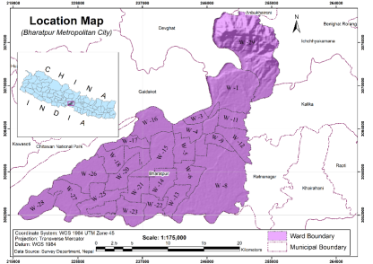
Figure 3. Location map of Bharatpur Metropolitan City.
2.2. Data Acquisition
Landsat 4-5 TM images from 1990, 2000, 2010, and 2020 were extracted from the administrative boundary of BMC. The images include seven spectral bands with a 30m spatial resolution, with a 120m spatial resolution. The scene spans 170 km north-south and 183 km east-west. Administrative boundary shapefiles were acquired from the Survey Department of Nepal, secondary data from Bharatpur Metropolitan City, and statistical data from the Central Bureau of Statistics.
2.3. Data Processing and Analysis
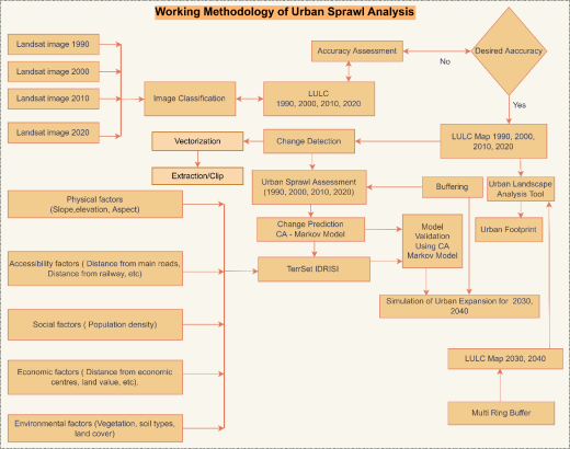
Figure 4. Schematic presentation of Methodology.
The study analyzed land use land cover patterns and changes from 1990 to 2020 using Landsat images and ERDAS IMAGINE and ArcGIS software. Accuracy assessments were conducted for 2030 and 2040, with models and urban footprint maps derived from the urban landscape analysis tool (ULAT). The following methodology describes the process of data preparation, analysis, and determination of the result for this study in Figure 4.
2.3.1. Image Classification
Landsat 5 TM and Landsat 8 OLI/TIRS imageries were classified using supervised pixel-based classification. Manual editing was used to create training areas for various classes, including agriculture land, barren land, built-up areas, forest land, and water bodies. Classified imageries were compared to Google Earth images and reclassified for area calculation. Land use land cover maps for years 1990, 2000, 2010, and 2020 were prepared. Image classification generates a raster file with class labels on each element. The actual quality of the images must be verified and quantified. Common sampling approaches include comparing classification results to a true world-class, using an error matrix for accuracy measures. Field observations yield the "true world-class," which is preferable. Reference sources are sometimes assumed to identify and compare class types. The ratio of equally classified pixels to pixels not classified is shown between reference and classification, with a value range of 0 to 1 (no agreement between reference and classification) to 1 (complete agreement between reference and classification).
2.3.2. Change Detection
Land use land cover changes from 1990 to 2020 were performed by the intersection of two LULC maps after vectorization of classified raster imageries. Land use changes were obtained after the intersection of two LULC maps.
2.3.3. Urban Sprawl Assessment
The study assessed urban sprawl between 1990 and 2020 using multi-ring buffer measurements and urban footprint measurements. A zero point was set near Hakim Chowk, and a 5 km incremental multiring buffer was created to identify sprawl levels. The graph of the incremental buffer versus built-up area provided a better understanding of urban spatial concentration and dispersion. The Urban Landscape Analysis Tool was used to identify types of urban sprawl in metropolitan cities, categorizing them into urban, water, and other data classes each year . The reclassified image was incorporated into ULAT, resulting in the creation of three output maps: urban footprint map, urban area map, and new development land cover map.
2.4. Urban Sprawl Extent Modeling
The study aimed to predict future land use and land cover in BMC from 1990 to 2020 using TerrSet Geospatial Monitoring and Modeling Software, which includes the Land Change Modeler (LCM). LCM simplifies land cover change analysis, allowing for quick analysis of changes in land cover and empirical modeling to explain variables and scenarios. The study also performed LULC change analysis between 1990 and 2020, focusing on urban sprawl changes and transition modeling from 1990 to 2010. The CA Markov chain analysis was used to divide the total area into a cell grid, representing an integrated area, and a grid or raster grid, representing a finite state . A modeled land use land cover map for 2020 was prepared using a transition model, land cover changes, and variables such as Digital Elevation Model, Slope, Aspect, Distance from River, Distance from Road, and Suitability map. Validation was performed using an earlier land cover image for LULC 2010 and later land cover change for LULC 2020, and urban extent for 2040 was prepared.
3. Results and Discussion
3.1. Land Use Land Cover
Land use and land cover are often used interchangeably, but each has distinct meanings. Land cover refers to the ground's surface, such as vegetation, urban infrastructure, water, or bare soil. Identifying land cover can aid in activities like thematic mapping and change detection analysis, while land use refers to land use for recreation, wildlife habitat, or farming. Land use planning (LULC) is influenced by various factors such as topography, lithology, soil type, rainfall, socio-cultural practices, and location. It involves abstracting features and grouping them into appropriate categories. Six different LULC maps were classified into five categories: agricultural land, barren land, built-up area, forest land, and water bodies. Classification is a methodical approach to grouping features and assigning relationships between them. Each LULC map was validate by performing accuracy assessment. All years of LULC area are presented below in Table 1.
Table 1. Land use land cover between 1990 – 2020 in BMC.

Year

1990

2000

2010

2020

Land Use

Area (Km2)

Agriculture Land

221.88

238.38

233.08

193.90

Barren Land

12.14

8.92

18.18

4.88

Built-up Area

3.29

6.79

17.28

64.32

Forest Land

192.08

174.98

159.70

164.02

Water Bodies

3.56

3.87

4.71

5.84

Figure 5 displays land use and land cover maps from 1990, 2000, 2010, and 2020, as depicted in (a), (b), (c), and (d) respectively. The majority of land in the metropolitan city is agricultural and cultivated, covering 221.88 km2 out of 432.95 km2. Forest land covers 44.36% of the total area, followed by barren land, which occupies 12.14 km2 and accounts for 2.80% of total land use land cover. Water bodies cover 3.56 km2, accounting for 0.82% of the total land use land cover. The built-up area occupies 0.76% of the total land use land cover, indicating a small built-up area in 1990. In 2000, agriculture and cultivated land occupied 55.06% of BMC's total land, followed by forest land at 174.98 km2, barren land at 8.92 km2, built-up area at 6.79 km2, and water bodies at 3.87 km2. The built-up area occupied the second-last small area in 1990, making it the second-smallest land cover in the metropolitan city. In 2010, agriculture and cultivated land occupied 53.84% of BMC's total land, followed by forest land, barren land, built-up area, and water bodies. The built-up area occupied 17.28 km2 of the total land use land cover, while water bodies occupied 4.71 km2. The built-up area occupied the second-last small area in the metropolitan city. In 2020, agriculture and cultivated land occupied 44.79% of BMC's total land, followed by forest land at 37.88%, built-up land at 14.86%, water bodies at 1.35%, and barren land at 1.13%. Built-up land was the second-smallest land cover in 2010, accounting for 1.13% of total land use.
3.2. Land Use Land Cover Change
The study reveals that built-up areas increased significantly in 2020, with agricultural land degradation and forest land degradation. The study also found that land cover changes from 1990 to 2020 were primarily agricultural, with most changes detected using a geospatial analysis tool.
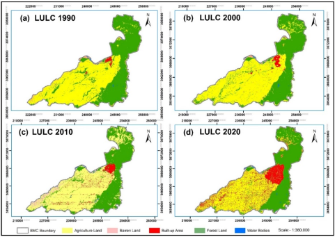
Figure 5. LULC maps for 1990, 2000, 2010, and 2020 of Bharatpur Metropolitan City.
The study reveals that the built-up area increased significantly in 2020 compared to previous years, primarily due to the degradation of agricultural land, forest land, and barren land near the river corridor. The agricultural land changes from 1990 to 2020 were 221.88 km2, 238.38 km2, 233.08 km2, and 193.90 km2, with most changes occurring from 2010 to 2020. Geospatial analysis tools were used to detect these changes. The study reveals that the built-up area increased significantly in 2020 compared to previous years, primarily due to the degradation of agricultural land, forest land, and barren land near the river corridor. The agricultural land changes from 1990 to 2020 were 221.88 km2, 238.38 km2, 233.08 km2, and 193.90 km2, with most changes occurring from 2010 to 2020. Geospatial analysis tools were used to detect these changes.
3.3. Types of Urban Sprawl
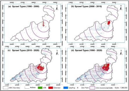
Figure 6. Urban sprawl types for the study period.
Urban sprawl types from 1990 to 2020 were depicted in Figure 6(a) shows urban sprawl types from 1990 to 2000, with expansion between infill and leapfrog development. From 1990 to 2000, 0.28 km2 of urbanized open area was infilled, with the maximum area of urbanization being 2.50 km2. Urban expansion primarily occurred within a 5 km buffer zone, with 2.47 km2 of extension growth detected, 0.03 km2 at 5-10 km, 0.29 km2 at 0-5 km, and 0.39 km2 at 0-20 km. Leapfrogging urban sprawl was also detected within this range. Figure 6(b) illustrates the urban sprawl types from 2000 to 2010. From 2000 to 2010, urbanization in urbanized open areas was primarily due to extension-type expansion within a 5 km buffer zone from zero point. The maximum area of urbanization was 5.50 km2, with 0.40 km2 of newly developed pixels being infill. The majority of urban expansion was due to extension-type expansion within this buffer zone. Leapfrogging type of urban sprawl was detected at (0-5) km proximity ranges, with a growth area of 2.03 km2.
Most of the growth was detected in infill types at BMC wards 2, 3, 10, and 11. Leapfrog type of sprawl was found in Fulbari, Gitanagar, Shivanagar, Patihani, and Mangalpur. Figure 6(c) illustrates the urban sprawl types from 2010 to 2020. In addition, from 2010 to 2020, Infill urban sprawl was the most prevalent, with 0.56 km2 of newly developed pixels in an urbanized open area. The maximum urbanization area was 26.80 km2. Figure 7 displays various types of urban sprawl within a 5 km incremental buffer from 1990 to 2020.
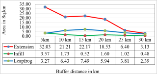
Figure 7. Types of Urban Sprawl within 5 km incremental buffer (1990 - 2020).
Most urban expansion occurred within a 5 km buffer zone from zero point, with 18.97 km2 of extension-type urban growth and 3.57 km2 at a 5-10 km proximity range. Infill urban sprawl occurred in newly constructed and widened roads, with most rural open land and agricultural land used for new settlements. Infill urban sprawl was mostly detected in BMC wards 2 and 11, while extension-type sprawl was mostly detected in BMC wards 3, 4, 7, 8, 9, 10, and 11. Leapfrog-type sprawl was detected in Fulbari, Gitanagar, Shivanagar, Patihani, and Mangalpur. From 1990 to 2020, 8.94 km2 of urbanization was infill, with the maximum area being 103.48 km2. Most urban expansion occurred within a 5 km buffer zone from zero point, with 32.03 km2 detected. Most of the city's land was arable and suitable for cereal crops, but rapid migration from rural areas transformed arable agriculture and cultivated land into built-up areas. Leapfrog expansion had a greater impact on cultivated and bare land, with leapfrog types of development dominating urban sprawl within 0 to 30 km buffer zones.
3.4. Urban Sprawl Modeling for 2030 and 2040
Urban sprawl extent modeling for 2030 and 2040 was done using TerrSet Geospatial Monitoring and Modeling Software and Land Change Modeler (LCM). Change probability grids for 2010 and 2020 were generated using LCM and CA-Markov chain analysis in TerrSet IDRISI software. The model divided the area into cell grids, representing finite states. Parameters for urban extent prediction included DEM, slope, distance from roads, rivers, aspect, and built-up suitability map. The LULC map for 2030 was created using the 2010 and 2020 LULC maps as a base year. The model state time (t1) and modeled state time (t2) were applied for land cover prediction in 2030 and 2040. The CA – CA-Markovian method was used, and the transition potential and transition area matrix were analyzed. Figure 8 shows the modeled LULC for BMC 2030 and 2040.
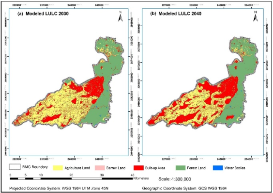
Figure 8. Modeled LULC of 2030 and 2040.
The 2030 LULC map of BMC shows forest land as the most dominant land, covering 160.29 km2 out of 432.95 km2, accounting for 37.02% of the total land. Agricultural land is the second dominant land, covering 149.98 km2, accounting for 34.64% of the total area. Built-up land is the third dominant land, covering 113.25 km2, accounting for 26.16% of the total land use land cover. Water bodies are the fourth dominant land cover, accounting for 1.33% of the total. Figure 8(a) demonstrates the built-up area in BMC has significantly increased from 3.29 km2 in 1990 to 64.32 km2 in 2020. This increase is expected to increase more than twofold from 1990 to 2030. However, there will be substantial decreases in agricultural and cultivated land, forest land, and barren land. Agriculture land is expected to decrease by 23%, barren land by 25%, forest land by 2%, and water bodies by 1%. Despite these changes, the built-up area is expected to increase by 76%. In 2040, forest land occupied 36.12% of the total land in BMC, covering 146.37 km2 out of 432.95 km2. The built-up area was the second dominant land, covering 34.49%. Agricultural land was the third dominant land, covering 27.43%. Water bodies were the fourth dominant land cover, covering 1.33%. The last dominant land cover was barren land, covering 0.62% of the total land use land cover. The modeled LULC map of BMC 2040 shows that bare and open land occupies a small area. The built-up area in BMC has increased by over twofold from 1990 to 2040, with substantial decreases in agricultural and cultivated land, forest land, and barren land.
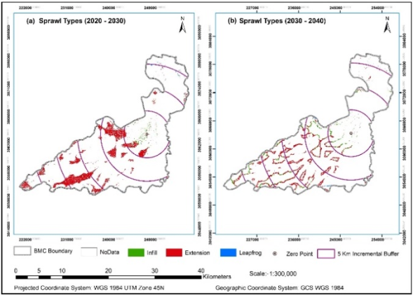
Figure 9. Types of Urban Sprawl from 2020 to 2040.
3.5. Types of Urban Sprawl from 2020 to 2040
From 2020 to 2030, urban expansion primarily occurred within a 10-kilometer buffer zone, with extension-type growth affecting 12.04 km2 of area, while "infill" expansion resulted in 0.96 km2 of growth. Figure 9 presents the types of urban sprawl from 2020 to 2040. Urban sprawl, characterized by rapid expansion within a buffer zone, is a significant aspect of urban growth. Detected from 0 km to 30 km, this type of expansion is mostly within a 10-km buffer zone. Out of the total urban expansion, 46 km2 is extension type, with red patches indicating growth in agriculture, rural development, and fringe open land. The majority of new development is sub-urban built-up and rural open land within 10 km and 15 km buffer zones. From 2030 to 2040, most urban expansion is extension type, with 8.01 km2 detected within 10-15 km proximity and 5.48 km2 at (5-10) km proximity. Infill-type expansion, on the other hand, results in a 1.43 km2 growth area.
3.6. Direction of Urban Sprawl
From 2010 to 2020, new built-up areas in the south-west and south-east zones of the city, including Gitanagar, Jyotinagar, Patihani, Dibyanagar, Sukranagar, Kadhaghari, and more, were concentrated due to high land value, urban road expansion, and rural facility increments. Figure 10 illustrates the direction of urban growth.
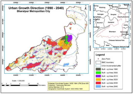
Figure 10. Direction of Urban Sprawl from 1990 to 2040.
4. Conclusion and Recommendations
4.1. Conclusion
The study analyzed urban sprawl in Bharatpur Metropolitan City from 1990 to 2040 using RS/GIS technology and techniques. The analysis revealed that the spatial distribution of built-up areas has rapidly grown, disoriented, and low efficiencies. New construction mainly occurred in suburbs and rural open land, with built-up areas occupying 3.29 km2 in 1990, 6.79 km2 in 2000, and 17.28 km2 in 2010. The agricultural and cultivated area decreased by more than three times compared to 2010, and barren and open land decreased from 12.14 km2 to 4.88 km2 between 1900 and 2020. The urban footprint map showed most new development was detected in the southeast and southwest zones from 2010 to 2020. The study concluded that the densification of settlement areas near existing built-up areas and the transformation of open and agricultural land into new settlements were the main causes of urbanization. Extension and leapfrogging are two major forms of urban sprawl, closely related to the BMC municipal division. The wards with high contribution of extension, infilling, and leapfrogging forms of urban expansion were distributed in the southeast and southwest zones from the main city. The study emphasizes the need for a balance between population growth and urbanization to improve the quality of life in the city.
4.2. Recommendations
The research analyzes urban sprawl in BMC from 1990 to 2040, predicting a significant increase in urbanization. This growth will have significant economic and environmental impacts. It highlights the need for better planning and land use planning to control urbanization and preserve the environment. The study also highlights the challenges of high population growth and urbanization, such as drainage issues, flooding, traffic congestion, and unplanned settlements. It emphasizes the need for government officials to protect river banks and natural environments for wildlife and habitats. Future studies should also consider environmental impacts like water pollution and climate change.
Abbreviations

AHP

Analytical Hierarchy Process

BMC

Bharatpur Metropolitan City

CA

Cellular Automata

CBS

Central Bureau of Statistics

DEM

Digital Elevation Model

GIS

Geographic Information System

LCM

Land Change Modeller

LULC

Land Use Land Cover

OLI

Operational Land Imager

RS

Remote Sensing

TIRS

Thermal Infrared Sensor

UGM

Urban Growth Model

ULAT

Urban Landscape Analysis Tool

Author Contributions
Sadhuram Lamichhane: Conceptualization, Data curation, Formal Analysis, Funding acquisition, Investigation, Methodology, Project administration, Resources, Software, Supervision, Validation, Visualization, Writing – original draft, Writing – review & editing
Conflicts of Interest
The author declares no conflicts of interest.
References
[1] B. Bhatta, “Analysis of Urban Growth and Sprawl from Remote Sensing Data,” pp. 14–26, Jan. 2010,
[2] S. Allah Yar, “Study of Urban Sprawl and its Social and Environmental Impacts on Urban Society in Latifabad Town, Hyderabad, Pakistan,” J Civil Environ Eng, vol. 07, no. 06, p. 6, 2017,
[3] R. M. Chitrakar, D. C. Baker, and M. Guaralda, “Urban growth and development of contemporary neighborhood public space in Kathmandu Valley, Nepal,” Habitat International, vol. 53, pp. 30–38, Apr. 2016,
[4] S. Bakrania, “Urbanisation and urban growth in Nepal,” GSDRC, University of Birmingham, Birmingham, UK: GSDRC, University of Birmingham., GSDRC Helpdesk Research Report, Oct. 2015. Accessed: Oct. 03, 2021. Available:
[5] G. Metternicht, A. Sabelli, and J. Spensley, “Climate change vulnerability, impact and adaptation assessment: Lessons from Latin America,” International Journal of Climate Change Strategies and Management, vol. 6, no. 4, pp. 442–476, Nov. 2014,
[6] BMC, “Welcome to Bharatpur Metropolitan City,” Bharatpur Metropolitan City Office of Municipal Executive, Bharatpur, 2018.
[7] CBS, “National Population and Housing Census 2011,” Nepal, National Report, 2011. Accessed: Mar. 15, 2021. Available:
[8] E. Muzzini and G. Aparicio, Urban Growth and Spatial Transition in Nepal. The World Bank, 2013.
[9] B. Antalyn and V. P. A. Weerasinghe, “Assessment of Urban Sprawl and Its Impacts on Rural Landmasses of Colombo District: A Study Based on Remote Sensing and GIS Techniques,” Asia-Pacific Journal of Rural Development, vol. 30, no. 1–2, pp. 139–154, Dec. 2020,
[10] B. Rimal, L. Zhang, D. Fu, R. Kunwar, and Y. Zhai, “Monitoring Urban Growth and the Nepal Earthquake 2015 for Sustainability of Kathmandu Valley, Nepal,” Land, vol. 6, no. 2, p. 42, Jun. 2017,
[11] Z. Shao, N. S. Sumari, A. Portnov, F. Ujoh, W. Musakwa, and P. J. Mandela, “Urban sprawl and its impact on sustainable urban development: a combination of remote sensing and social media data,” Geo-spatial Information Science, pp. 1–15, Jul. 2020,
[12] B. S. Almeida, “A GIS Assessment of Urban Sprawl in Richmond, Virginia,” Virginia Polytechnic Institute and State University, Blacksburg, VA 24060 10 May 2005, 2005. Accessed: May 03, 2020. Available:
[13] L. Gervasoni, M. Bosch, S. Fenet, and P. Sturm, “Calculating spatial urban sprawl indices using open data,” p. 23, 2017.
[14] N. Falah, A. Karimi, and A. T. Harandi, “Urban growth modeling using cellular automata model and AHP (case study: Qazvin city),” Model. Earth Syst. Environ., vol. 6, no. 1, pp. 235–248, Mar. 2020,
[15] T. Litman, “Analysis of Public Policies That Unintentionally Encourage and Subsidize Urban Sprawl,” Victoria Transport Policy Institute, Canada, Mar. 2015. Accessed: May 03, 2021. Available:
[16] W. Suwal, “A Study of Land Use Planning Practices and the Relationship Between Population Distribution and Transportation Infrastructure in Kathmandu, Nepal.” p. 95, 2009.
[17] H. B. Wakode, “Analysis of Urban Growth and Assessment of Impact of Urbanization on Water Resources- A Case Study of Hyderabad, India,” RWTH Aachen University, Templergraben 55, 52062 Aachen, Germany, 2016. Accessed: Apr. 15, 2021. Available:
[18] R. Pendall, “Do Land-Use Controls Cause Sprawl?,” Environment and Planning B: Planning and Design, vol. 26, no. 4, pp. 555–571, 1999,
[19] J. Carruthers and G. Ulfarsson, “Fragmentation and Sprawl: Evidence from Interregional Analysis,” Growth and Change, vol. 33, pp. 312–340, Jun. 2002,
[20] J. K. Brueckner, “Urban Sprawl: Diagnosis and Remedies,” International Regional Science Review, vol. 23, no. 2, pp. 160–171, Apr. 2000,
[21] S. Jaquet, T. Kohler, and G. Schwilch, “Labour Migration in the Middle Hills of Nepal: Consequences on Land Management Strategies,” Sustainability, vol. 11, no. 5, pp. 1–19, Mar. 2019,
[22] T. Noszczyk, “A review of approaches to land use changes modeling,” Human and Ecological Risk Assessment, vol. 25, pp. 1377–1405, Aug. 2019,
[23] A. Ishtiaque, M. Shrestha, and N. Chhetri, “Rapid Urban Growth in the Kathmandu Valley, Nepal: Monitoring Land Use Land Cover Dynamics of a Himalayan City with Landsat Imageries,” Environments, vol. 4, no. 4, p. 72, Oct. 2017,
[24] P. H. Verburg et al., “Land system science and sustainable development of the earth system: A global land project perspective,” Anthropocene, vol. 12, pp. 29–41, 2015,
[25] O. Gillham, O. G. A. S. MacLean, A. S. MacLean, and I. Press, The Limitless City: A Primer on the Urban Sprawl Debate. Island Press, 2002. Available:
[26] T. Zhang, “Community features and urban sprawl: the case of the Chicago metropolitan region,” Land Use Policy, vol. 18, no. 3, pp. 221–232, 2001,
[27] M. Kasanko et al., “Are European cities becoming dispersed?: A comparative analysis of 15 European urban areas,” Landscape and Urban Planning, vol. 77, no. 1, pp. 111–130, 2006,
[28] G. Galster, R. Hanson, M. Ratcliffe, H. Wolman, S. Coleman, and J. Freihage, “Wrestling Sprawl to the Ground: Defining and Measuring an Elusive Concept,” Housing Policy Debate, vol. 12, pp. 681–717, 2001,
[29] P. Nikolov, “A Survey of Bulgarian (National) Planning and Regulation Acts and Documents Concerning Urban Sprawl,” presented at the 2nd International Scientific Conference, Bulgaria, May 2013, pp. 2–12. Available:
[30] P. Christiansen and T. Loftsgarden, “Drivers behind urban sprawl in Europe,” Institute of Transport Economics (TØI), pp. 1–29, 2011.
[31] R. B. Thapa and Y. Murayama, “Scenario-based urban growth allocation in Kathmandu Valley, Nepal,” Landscape and Urban Planning, vol. 105, no. 1–2, pp. 140–148, Mar. 2012,
[32] X. Li, L. Yang, Y. Ren, H. Li, and Z. Wang, “Impacts of Urban Sprawl on Soil Resources in the ChangchunJilin Economic Zone, China, 20002015,” Int J Environ Res Public Health, vol. 15, no. 6, p. 1186, Jun. 2018,
[33] K. Lynch, Theory of Good City, 2nd ed. MIT Press, Cambridge, MA, 1984. Available:
[34] L. Feyen and R. Dankers, “Impact of global warming on streamflow drought in Europe,” J. Geophys. Res., vol. 114, no. D17, pp. 1–17, Sep. 2009,
[35] J. R. Kenworthy and F. B. Laube, “Patterns of automobile dependence in cities: an international overview of key physical and economic dimensions with some implications for urban policy,” Transportation Research Part A: Policy and Practice, vol. 33, no. 7–8, pp. 691–723, 1999.
[36] J. Hirschhorn, “Environment, Quality of Life, and Urban Growth in the New Economy,” Environmental Quality Management, vol. 10, pp. 1–8, Apr. 2001,
[37] M. Kahn, “The Environmental Impact of Suburbanization,” Journal of Policy Analysis and Management, vol. 19, pp. 569–586, Sep. 2000,
[38] T. J. Nechyba and R. P. Walsh, “Urban Sprawl,” Journal of Economic Perspectives, vol. 18, no. 4, pp. 177–200, 2004.
[39] R. B. Thapa and Y. Murayama, “Urban growth modeling of Kathmandu metropolitan region, Nepal,” Computers, Environment, and Urban Systems, vol. 35, no. 1, pp. 25–34, Jan. 2011,
[40] C. Xu, M. Liu, C. Zhang, S. An, W. Yu, and J. M. Chen, “The spatiotemporal dynamics of rapid urban growth in the Nanjing metropolitan region of China,” Landscape Ecol, vol. 22, no. 6, pp. 925–937, May 2007,
[41] R. A. Francis and M. A. Chadwick, “Urban Ecosystems Understanding the Human Environment,” London, Mar. 2013,
[42] C. Dietzel, M. Herold, J. J. Hemphill, and K. C. Clarke, “Spatio‐temporal dynamics in California’s Central Valley: Empirical links to urban theory,” International Journal of Geographical Information Science, vol. 19, no. 2, pp. 175–195, 2005,
[43] G.-J. Knaap and E. Talen, “New Urbanism and Smart Growth: A Few Words from the Academy,” International Regional Science Review - INT REG SCI REV, vol. 28, pp. 107–118, Apr. 2005,
[44] Y. Song and G.-J. Knaap, “Measuring Urban Form: Is Portland Winning the War on Sprawl?,” Journal of the American Planning Association, vol. 70, pp. 210–225, Jun. 2004,
[45] Y. Song, “Smart Growth and Urban Development Pattern: A Comparative Study,” International Regional Science Review, vol. 28, pp. 239–265, Apr. 2005,
[46] F. K. Benfield, M. Raimi, and D. Chen, “Once There Were Greenfields: How Urban Sprawl is Undermining America’s Environment, Economy, and Social Fabric,” 1999.
[47] R. E. Heimlich and W. D. Anderson, “Development at the Urban Fringe and Beyond: Impacts on Agriculture and Rural Land,” p. 88, 2001.
[48] Torrens and Alberti - Measuring Sprawl.
[49] Y.-H. Tsai, “Quantifying Urban Form: Compactness versus ‘Sprawl,’” Urban Studies, vol. 42, no. 1, pp. 141–161, Jan. 2005,
[50] S. Angel, J. Parent, and D. Civco, “Urban Sprawl Metrics: An Analysis of Global Urban Expansion Using GIS,” p. 12, 2007.
[51] M. Batty, E. Besussi, and N. Chin, “Traffic, urban growth, and suburban sprawl,” 2003.
[52] E. Besussi, N. Chin, M. Batty, and P. Longley, “Chapter 2 The Structure and Form of Urban Settlements,” 2017.
[53] R. P. Jason, “Urban Landscape Analysis Tool,” Center for Land Use Education & Research, 2009.
[54] P. M. Torrens and M. Alberti, “Measuring Sprawl,” p. 34.
[55] L. A. Mantelas, P. Prastacos, and T. Hatzichristos, “Modeling Urban Growth using Fuzzy Cellular Automata,” p. 12, 2008.
[56] Y. Feng, Y. Liu, X. Tong, M. Liu, and S. Deng, “Modeling dynamic urban growth using cellular automata and particle swarm optimization rules,” Landscape and Urban Planning - LANDSCAPE URBAN PLAN, vol. 102, pp. 188–196, Sep. 2011,
[57] A. E. Pravitasari, E. Rustiadi, S. P. Mulya, Y. Setiawan, L. N. Fuadina, and A. Murtadho, “Identifying the driving forces of urban expansion and its environmental impact in Jakarta-Bandung mega-urban region,” IOP Conf. Ser.: Earth Environ. Sci., vol. 149, p. 012044, May 2018,
[58] K. Kityuttachai, N. Tripathi, T. Tipdecho, and R. Shrestha, “CA-Markov Analysis of Constrained Coastal Urban Growth Modeling: Hua Hin Seaside City, Thailand,” Sustainability, vol. 5, no. 4, pp. 1480–1500, Apr. 2013,
[59] P. K. Mallupattu and J. R. Sreenivasula Reddy, “Analysis of Land Use/Land Cover Changes Using Remote Sensing Data and GIS at an Urban Area, Tirupati, India,” The Scientific World Journal, vol. 2013, pp. 1–6, 2013,
Cite This Article
  • APA Style

    Lamichhane, S. (2026). Geospatial Modeling of Urban Sprawl in Bharatpur Metropolitan City. Urban and Regional Planning, 11(2), 96-109. https://doi.org/10.11648/j.urp.20261102.11

    Copy | Download

    ACS Style

    Lamichhane, S. Geospatial Modeling of Urban Sprawl in Bharatpur Metropolitan City. Urban Reg. Plan. 2026, 11(2), 96-109. doi: 10.11648/j.urp.20261102.11

    Copy | Download

    AMA Style

    Lamichhane S. Geospatial Modeling of Urban Sprawl in Bharatpur Metropolitan City. Urban Reg Plan. 2026;11(2):96-109. doi: 10.11648/j.urp.20261102.11

    Copy | Download

  • @article{10.11648/j.urp.20261102.11,
      author = {Sadhuram Lamichhane},
      title = {Geospatial Modeling of Urban Sprawl in Bharatpur Metropolitan City},
      journal = {Urban and Regional Planning},
      volume = {11},
      number = {2},
      pages = {96-109},
      doi = {10.11648/j.urp.20261102.11},
      url = {https://doi.org/10.11648/j.urp.20261102.11},
      eprint = {https://article.sciencepublishinggroup.com/pdf/10.11648.j.urp.20261102.11},
      abstract = {Rapid socioeconomic developments have spurred urban sprawl in Nepal. Bharatpur Metropolitan City (BMC) in recent decades, resulting in notable changes to the land use and environment. Using Landsat images and GIS-based methods, this study examines the spatial and temporal dynamics of urban sprawl from 1990 to 2020 and projects future growth through 2040. Built-up areas expanded by over 20 times, from 3.29 km2 in 1990 to 64.32 km2 in 2020, according to the Land Use and Land Cover (LULC) categorization. At the same time, there was a significant amount of land conversion as agricultural land decreased from 221.88 km2 to 193.90 km2 and barren land decreased by more than 60%. Three predominant types of urban sprawl were found: leapfrog (important within 0–30 km buffers), infill (8.94 km2), and extension (103.48 km2). The most common areas for extension-type sprawl were those between 0 and 5 km. Built-up area is expected to rise by 132% from 2020 levels to 113.25 km2 by 2030 and 149.33 km2 by 2040, according to spatiotemporal analysis and CA-Markov modelling. By 2040, this growth is expected to further reduce the amount of agricultural land to 118.78 km2. These results underline how urgently urban planning interventions are needed to manage haphazard development, protect arable land, and direct sustainable growth. The study shows how important it is to combine predictive modelling, spatial analysis, and remote sensing to inform land use regulations in areas that are rapidly becoming more urbanized.},
     year = {2026}
    }
    

    Copy | Download

  • TY  - JOUR
    T1  - Geospatial Modeling of Urban Sprawl in Bharatpur Metropolitan City
    AU  - Sadhuram Lamichhane
    Y1  - 2026/04/28
    PY  - 2026
    N1  - https://doi.org/10.11648/j.urp.20261102.11
    DO  - 10.11648/j.urp.20261102.11
    T2  - Urban and Regional Planning
    JF  - Urban and Regional Planning
    JO  - Urban and Regional Planning
    SP  - 96
    EP  - 109
    PB  - Science Publishing Group
    SN  - 2575-1697
    UR  - https://doi.org/10.11648/j.urp.20261102.11
    AB  - Rapid socioeconomic developments have spurred urban sprawl in Nepal. Bharatpur Metropolitan City (BMC) in recent decades, resulting in notable changes to the land use and environment. Using Landsat images and GIS-based methods, this study examines the spatial and temporal dynamics of urban sprawl from 1990 to 2020 and projects future growth through 2040. Built-up areas expanded by over 20 times, from 3.29 km2 in 1990 to 64.32 km2 in 2020, according to the Land Use and Land Cover (LULC) categorization. At the same time, there was a significant amount of land conversion as agricultural land decreased from 221.88 km2 to 193.90 km2 and barren land decreased by more than 60%. Three predominant types of urban sprawl were found: leapfrog (important within 0–30 km buffers), infill (8.94 km2), and extension (103.48 km2). The most common areas for extension-type sprawl were those between 0 and 5 km. Built-up area is expected to rise by 132% from 2020 levels to 113.25 km2 by 2030 and 149.33 km2 by 2040, according to spatiotemporal analysis and CA-Markov modelling. By 2040, this growth is expected to further reduce the amount of agricultural land to 118.78 km2. These results underline how urgently urban planning interventions are needed to manage haphazard development, protect arable land, and direct sustainable growth. The study shows how important it is to combine predictive modelling, spatial analysis, and remote sensing to inform land use regulations in areas that are rapidly becoming more urbanized.
    VL  - 11
    IS  - 2
    ER  - 

    Copy | Download

Author Information
  • Abstract
  • Keywords
  • Document Sections

    1. 1. Introduction
    2. 2. Material and Methods
    3. 3. Results and Discussion
    4. 4. Conclusion and Recommendations
    Show Full Outline
  • Abbreviations
  • Author Contributions
  • Conflicts of Interest
  • References
  • Cite This Article
  • Author Information